GPT in words and code

I find that the best way to understand how machine learning papers work is to write the code for a model forward pass. If you can load the weights from a pre-trained model and get the same outputs from a single model inference, you can be pretty confident that you’ve re-implemented all of the details from a model. The advantages of doing this are:

Does not require any training, which can be time-consuming and expensive.
Can test model outputs layer-by-layer to validate the correctness of different components.
Get a satisfying payoff at the end with a working model, and develop an understanding of the model that is more detailed than what is found in the paper.

This is the strategy adopted in Jay Mody’s picoGPT and Andrej Karpathy’s nanoGPT.

For a good exercise to replicate GPT-inference, I would recommend reimplementing the gpt2 function in the picoGPT repo above, located here. picoGPT makes this especially easy because the weight loading code is already written and you can just write the forward pass in NumPy. A link to my implementation can be found here.

Model architecture #

Here I will break down the GPT architecture into its components. Here I will focus on GPT-2, since the weights are publicly available. GPT-3 has a very similar architecture but is massively scaled up.

GPT2 can be implemented in the following pseudocode:

def gpt(input_string):
  input_tokens = tokenize(input_string)
  x = wte[input_tokens] + wpe[range(len(input_tokens))]
  for transformer_block in transformer_blocks:
    x = transformer_block(x) 
  x = layer_norm(x)
  return x @ wte.T

In the following sections we will break down each piece.

1) Byte-Pair Embedding Tokenizer #

$\text{String} -> \text{List[Integer]}$

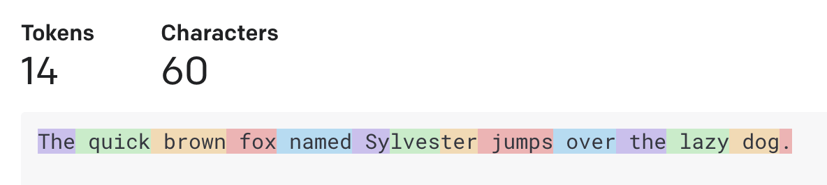
The first step is to convert words to numbers using a tokenizer. GPT uses byte-pair encoding (BPE). In BPE, the most common words are mapped to single tokens while less common words will be broken down into chunks and mapped to multiple tokens.

OpenAI’s Tokenizer tool shows how different sentences will be broken into tokens under BPE. In this example, most words get mapped to a single token, except for “Sylvester,” which gets chunked into three tokens: Sy, lves, and ter.

Tokenizer

2.1) Word Embeddings #

We start by embedding each token which is done with a lookup

wte[input_tokens].

This gives us a tensor of shape $n_{tokens} \times n_{embed}$ . For GPT-2, $n_{embed} = 1600$ .

2.2) Positional Encodings #

Transformers are invariant to the order of inputs, so we need to tell the model which position each word is in. We grab positional embeddings with a similar lookup:

wpe[range(len(inputs))]

This gives us another tensor of shape $n_{tokens} \times n_{embed}$ .

2.3) Sum #

Now we simply sum of the two tensors from before to get a single tensor of shape $n_{tokens} \times n_{embed}$ .

x = wte[inputs] + wpe[range(len(inputs))]

3) Transformer Block #

The transformer block can be expressed as the following operation:

def transformer_block(x):
  x = x + MultiHeadAttention(LayerNorm(x))
  x = x = FFN(LayerNorm(x))
  return x

3.1) Attention #

We will start by discussing single-head attention. We define the attention operation as follows: $$ \text{Attention}(\mathbf{Q}, \mathbf{K}, \mathbf{V}) = \text{softmax} \left ( \frac{\mathbf{QK^T}}{\sqrt{d_k}} \right ) \mathbf{V}. $$

Here, $\mathbf{Q}, \mathbf{K}, \mathbf{V}$ are obtained from a linear layer on the input tensor.

In code, this looks like this:

causal_mask = (1 - np.tri(x.shape[0], dtype=x.dtype)) * -1e10

def attention(q, k, v, mask):
    # [n_q, d_k], [n_k, d_k], [n_k, d_v], [n_q, n_k] -> [n_q, d_v]
    return softmax(q @ k.T / np.sqrt(q.shape[-1]) + mask) @ v

Here, the causal mask prevents a tokens from attending to future tokens - in the context of language modeling, this is necessary since we will see each word stream in one by one.

Intuitively, $\mathbf{Q} \mathbf{K}^T$ will result in an “importance” matrix that returns the importance of each token to each other token. We then divide this by $\sqrt{d_k}$ and then pass this through a softmax. Finally, we multiply this by the $\mathbf{V}$ matrix, which represents the importance of each token.

3.2) MultiHeadAttention #

MultiHeadAttention is a simple extension of single-head attention. Here, we will just redo the above operation several times with a different learned $\mathbf{Q}, \mathbf{K}$ and $\mathbf{V}$ matrices. We will then concatenate the result of each attention head together, which is then multiplied by a linear projection.

In code, this looks like this:

def multi_head_attention(x, c_attn, c_proj, n_head):
    x = linear(x,
               w=c_attn['w'],
               b=c_attn['b'])

    qkv = np.split(x, 3, axis=-1)

    qkv_heads = []
    for elt in qkv:
        qkv_head_split = np.split(elt, n_head, axis=-1)
        qkv_heads.append(qkv_head_split)

    causal_mask = (1 - np.tri(x.shape[0], dtype=x.dtype)) * -1e10

    out_heads = []
    for q, k, v in zip(*qkv_heads):
        x = attention(q, k, v, causal_mask)
        out_heads.append(x)
    
    x = np.hstack(out_heads)

    x = linear(x,
               w=c_proj['w'],
               b=c_proj['b'])

    return x

4) FFN #

The rest of the transformer block is quite simple. The FFN block looks like this:

def ffn(x):
  x = linear(x) # project up
  x = gelu(x)
  x = linear(x) # project down

The GELU is an activation function defined in this paper, defined as $x \Phi(x)$ , where $\Phi(x)$ is the standard Gaussian CDF function.

We will call the FFN block in the transformer block with a skip connection as follows:

x = x + ffn(x)

5) LayerNorm and Decode #

Before decoding words, we will run a last iteration of LayerNorm as follows:

x = x + layer_norm(x)

At the end, we have a big word embedding matrix. We decode by multiplying by the transpose of $W_E$ to get back to tokens:

x = x @ wte.T

Demo #

And that’s it! For a demo, check out my repo. https://github.com/acganesh/tinyGPT/